
Machine Learning (6) - 분류 평가 지표
평가
정밀도와 재현율
In [1]:
def get_clf_eval(y_test, pred):
    from sklearn.metrics import accuracy_score, precision_score, recall_score, confusion_matrix
    confusion = confusion_matrix(y_test, pred)
    accuracy = accuracy_score(y_test, pred)
    precision = precision_score(y_test, pred)
    recall = recall_score(y_test, pred)
    print('==오차 행렬==')
    print(confusion)
    print(f"정확도: {accuracy:.4f}, 정밀도: {precision:.4f}, 재현율: {recall:.4f}")
In [2]:
import pandas as pd
import numpy as np
from sklearn.model_selection import train_test_split
from sklearn.linear_model import LogisticRegression
In [3]:
# Null 처리 함수
def fillna(df):
    df['Age'].fillna(df['Age'].mean(), inplace=True)
    df['Cabin'].fillna('N', inplace=True)
    df['Embarked'].fillna('N', inplace=True)
    df['Fare'].fillna('0', inplace=True)
    return df

# 불필요한 feature 제거
def drop_features(df):
    df.drop(['PassengerId', 'Name', 'Ticket'], axis=1, inplace=True)
    return df

# 레이블 인코딩
def format_features(df):
    from sklearn.preprocessing import LabelEncoder
    df['Cabin'] = df['Cabin'].str[:1]
    features = ['Sex', 'Cabin', 'Embarked']
    for feature in features:
        le = LabelEncoder()
        df[feature] = le.fit_transform(df[feature])
        print(le.classes_)
    return df

# 데이터 전처리 함수 전체 호출
def transform_features(df):
    df = fillna(df)
    df = drop_features(df)
    df = format_features(df)
    return df
In [4]:
df = pd.read_csv('titanic.csv')
y = df['Survived']
X = df.drop(columns=['Survived']) # 원본 적용 안함
X = transform_features(X)
Out [4]:
['female' 'male']
['A' 'B' 'C' 'D' 'E' 'F' 'G' 'N' 'T']
['C' 'N' 'Q' 'S']
In [5]:
X_train, X_test, y_train, y_test = train_test_split(X, y, test_size=0.2, random_state=11)
In [6]:
lr_clf = LogisticRegression(solver='liblinear')
lr_clf.fit(X_train, y_train)
pred = lr_clf.predict(X_test)
get_clf_eval(y_test, pred)
Out [6]:
==오차 행렬==
[[108  10]
 [ 14  47]]
정확도: 0.8659, 정밀도: 0.8246, 재현율: 0.7705
정밀도/재현율 트레이드오프
In [7]:
pred
Out [7]:
array([1, 0, 0, 0, 0, 0, 0, 1, 0, 1, 0, 0, 0, 0, 0, 0, 0, 0, 0, 1, 0, 0,
       0, 0, 0, 0, 0, 0, 0, 0, 1, 1, 0, 1, 0, 0, 0, 1, 0, 0, 0, 0, 1, 1,
       1, 1, 1, 0, 1, 0, 0, 0, 0, 1, 0, 0, 0, 0, 0, 0, 0, 0, 0, 0, 0, 0,
       1, 1, 1, 0, 0, 0, 0, 1, 0, 0, 0, 0, 1, 0, 1, 1, 1, 0, 1, 1, 0, 0,
       1, 0, 0, 0, 0, 0, 1, 0, 1, 0, 0, 1, 1, 0, 1, 0, 1, 0, 0, 0, 0, 0,
       0, 0, 0, 1, 0, 0, 0, 0, 1, 0, 0, 0, 0, 0, 0, 0, 0, 0, 1, 0, 1, 0,
       1, 1, 1, 0, 1, 0, 0, 1, 1, 0, 0, 0, 0, 1, 0, 0, 1, 0, 0, 1, 1, 0,
       1, 1, 0, 0, 1, 1, 0, 1, 0, 1, 0, 1, 1, 0, 0, 1, 0, 1, 0, 0, 0, 0,
       0, 0, 1], dtype=int64)
In [8]:
pred_proba = lr_clf.predict_proba(X_test) # 각각의 데이터별 [0이 될 확률, 1이 될 확률] # 임곗값(Threshold) 0.5를 기준으로
In [9]:
np.concatenate([pred_proba, pred.reshape(-1, 1)], axis=1) # pred의 모양을 바꿔줘야한다 # axis=1 컬럼단위로 붙임
Out [9]:
array([[0.44935225, 0.55064775, 1.        ],
       [0.86335511, 0.13664489, 0.        ],
       [0.86429643, 0.13570357, 0.        ],
       [0.84968519, 0.15031481, 0.        ],
       [0.82343409, 0.17656591, 0.        ],
       [0.84231224, 0.15768776, 0.        ],
       [0.87095489, 0.12904511, 0.        ],
       [0.27228603, 0.72771397, 1.        ],
       [0.78185128, 0.21814872, 0.        ],
       [0.33185998, 0.66814002, 1.        ],
       [0.86178763, 0.13821237, 0.        ],
       [0.87058097, 0.12941903, 0.        ],
       [0.8642595 , 0.1357405 , 0.        ],
       [0.87065944, 0.12934056, 0.        ],
       [0.56033544, 0.43966456, 0.        ],
       [0.85003022, 0.14996978, 0.        ],
       [0.88954172, 0.11045828, 0.        ],
       [0.74250732, 0.25749268, 0.        ],
       [0.71120224, 0.28879776, 0.        ],
       [0.23776278, 0.76223722, 1.        ],
       [0.75684107, 0.24315893, 0.        ],
       [0.62428169, 0.37571831, 0.        ],
       [0.84655246, 0.15344754, 0.        ],
       [0.82711256, 0.17288744, 0.        ],
       [0.86825628, 0.13174372, 0.        ],
       [0.77003828, 0.22996172, 0.        ],
       [0.82946349, 0.17053651, 0.        ],
       [0.90336131, 0.09663869, 0.        ],
       [0.73372049, 0.26627951, 0.        ],
       [0.68847387, 0.31152613, 0.        ],
       [0.07646869, 0.92353131, 1.        ],
       [0.2253212 , 0.7746788 , 1.        ],
       [0.87161939, 0.12838061, 0.        ],
       [0.24075418, 0.75924582, 1.        ],
       [0.62711731, 0.37288269, 0.        ],
       [0.77003828, 0.22996172, 0.        ],
       [0.90554276, 0.09445724, 0.        ],
       [0.40602574, 0.59397426, 1.        ],
       [0.93043584, 0.06956416, 0.        ],
       [0.8765052 , 0.1234948 , 0.        ],
       [0.69797422, 0.30202578, 0.        ],
       [0.89664595, 0.10335405, 0.        ],
       [0.21993379, 0.78006621, 1.        ],
       [0.31565713, 0.68434287, 1.        ],
       [0.37942228, 0.62057772, 1.        ],
       [0.37932891, 0.62067109, 1.        ],
       [0.07161281, 0.92838719, 1.        ],
       [0.55777586, 0.44222414, 0.        ],
       [0.07914487, 0.92085513, 1.        ],
       [0.86803082, 0.13196918, 0.        ],
       [0.50790057, 0.49209943, 0.        ],
       [0.87065944, 0.12934056, 0.        ],
       [0.85576405, 0.14423595, 0.        ],
       [0.34870129, 0.65129871, 1.        ],
       [0.71558417, 0.28441583, 0.        ],
       [0.78853206, 0.21146794, 0.        ],
       [0.7461921 , 0.2538079 , 0.        ],
       [0.86429   , 0.13571   , 0.        ],
       [0.84079003, 0.15920997, 0.        ],
       [0.59838066, 0.40161934, 0.        ],
       [0.73532081, 0.26467919, 0.        ],
       [0.88705596, 0.11294404, 0.        ],
       [0.545528  , 0.454472  , 0.        ],
       [0.55326343, 0.44673657, 0.        ],
       [0.62583522, 0.37416478, 0.        ],
       [0.88363277, 0.11636723, 0.        ],
       [0.35181256, 0.64818744, 1.        ],
       [0.39903352, 0.60096648, 1.        ],
       [0.08300815, 0.91699185, 1.        ],
       [0.85072522, 0.14927478, 0.        ],
       [0.86778819, 0.13221181, 0.        ],
       [0.83070924, 0.16929076, 0.        ],
       [0.87649042, 0.12350958, 0.        ],
       [0.05959915, 0.94040085, 1.        ],
       [0.78735759, 0.21264241, 0.        ],
       [0.87065944, 0.12934056, 0.        ],
       [0.716541  , 0.283459  , 0.        ],
       [0.79159804, 0.20840196, 0.        ],
       [0.20303098, 0.79696902, 1.        ],
       [0.86429   , 0.13571   , 0.        ],
       [0.2400505 , 0.7599495 , 1.        ],
       [0.37123587, 0.62876413, 1.        ],
       [0.08369626, 0.91630374, 1.        ],
       [0.84018612, 0.15981388, 0.        ],
       [0.07766719, 0.92233281, 1.        ],
       [0.08973248, 0.91026752, 1.        ],
       [0.84723076, 0.15276924, 0.        ],
       [0.8624153 , 0.1375847 , 0.        ],
       [0.16539734, 0.83460266, 1.        ],
       [0.87065944, 0.12934056, 0.        ],
       [0.87065944, 0.12934056, 0.        ],
       [0.77003828, 0.22996172, 0.        ],
       [0.75416744, 0.24583256, 0.        ],
       [0.87065944, 0.12934056, 0.        ],
       [0.37932891, 0.62067109, 1.        ],
       [0.89883889, 0.10116111, 0.        ],
       [0.07361403, 0.92638597, 1.        ],
       [0.87897226, 0.12102774, 0.        ],
       [0.60197825, 0.39802175, 0.        ],
       [0.06738996, 0.93261004, 1.        ],
       [0.47948281, 0.52051719, 1.        ],
       [0.9046927 , 0.0953073 , 0.        ],
       [0.05673721, 0.94326279, 1.        ],
       [0.88180787, 0.11819213, 0.        ],
       [0.45587969, 0.54412031, 1.        ],
       [0.86133437, 0.13866563, 0.        ],
       [0.84974929, 0.15025071, 0.        ],
       [0.85072697, 0.14927303, 0.        ],
       [0.55502751, 0.44497249, 0.        ],
       [0.88426898, 0.11573102, 0.        ],
       [0.84747418, 0.15252582, 0.        ],
       [0.87269562, 0.12730438, 0.        ],
       [0.67538692, 0.32461308, 0.        ],
       [0.48275247, 0.51724753, 1.        ],
       [0.86825628, 0.13174372, 0.        ],
       [0.9159719 , 0.0840281 , 0.        ],
       [0.84194204, 0.15805796, 0.        ],
       [0.78872838, 0.21127162, 0.        ],
       [0.11141754, 0.88858246, 1.        ],
       [0.90534855, 0.09465145, 0.        ],
       [0.87071643, 0.12928357, 0.        ],
       [0.86905438, 0.13094562, 0.        ],
       [0.91525793, 0.08474207, 0.        ],
       [0.58196827, 0.41803173, 0.        ],
       [0.98025012, 0.01974988, 0.        ],
       [0.87071643, 0.12928357, 0.        ],
       [0.87219019, 0.12780981, 0.        ],
       [0.7119464 , 0.2880536 , 0.        ],
       [0.34348899, 0.65651101, 1.        ],
       [0.70226693, 0.29773307, 0.        ],
       [0.06738996, 0.93261004, 1.        ],
       [0.59805546, 0.40194454, 0.        ],
       [0.3288534 , 0.6711466 , 1.        ],
       [0.48644765, 0.51355235, 1.        ],
       [0.42864813, 0.57135187, 1.        ],
       [0.56346572, 0.43653428, 0.        ],
       [0.25853148, 0.74146852, 1.        ],
       [0.77643225, 0.22356775, 0.        ],
       [0.87632447, 0.12367553, 0.        ],
       [0.15009277, 0.84990723, 1.        ],
       [0.13434695, 0.86565305, 1.        ],
       [0.85072697, 0.14927303, 0.        ],
       [0.86772102, 0.13227898, 0.        ],
       [0.89628756, 0.10371244, 0.        ],
       [0.88613339, 0.11386661, 0.        ],
       [0.34797639, 0.65202361, 1.        ],
       [0.89917048, 0.10082952, 0.        ],
       [0.72997342, 0.27002658, 0.        ],
       [0.12221446, 0.87778554, 1.        ],
       [0.8171969 , 0.1828031 , 0.        ],
       [0.61865112, 0.38134888, 0.        ],
       [0.37370305, 0.62629695, 1.        ],
       [0.38348341, 0.61651659, 1.        ],
       [0.86463298, 0.13536702, 0.        ],
       [0.25161298, 0.74838702, 1.        ],
       [0.10388332, 0.89611668, 1.        ],
       [0.57648057, 0.42351943, 0.        ],
       [0.85476848, 0.14523152, 0.        ],
       [0.31415125, 0.68584875, 1.        ],
       [0.33907972, 0.66092028, 1.        ],
       [0.84347719, 0.15652281, 0.        ],
       [0.23261134, 0.76738866, 1.        ],
       [0.88859273, 0.11140727, 0.        ],
       [0.35220567, 0.64779433, 1.        ],
       [0.58554858, 0.41445142, 0.        ],
       [0.36143288, 0.63856712, 1.        ],
       [0.1363406 , 0.8636594 , 1.        ],
       [0.67797005, 0.32202995, 0.        ],
       [0.88600083, 0.11399917, 0.        ],
       [0.13946115, 0.86053885, 1.        ],
       [0.87095489, 0.12904511, 0.        ],
       [0.20616022, 0.79383978, 1.        ],
       [0.76719902, 0.23280098, 0.        ],
       [0.77437244, 0.22562756, 0.        ],
       [0.50324048, 0.49675952, 0.        ],
       [0.91079838, 0.08920162, 0.        ],
       [0.84970738, 0.15029262, 0.        ],
       [0.54874087, 0.45125913, 0.        ],
       [0.48192063, 0.51807937, 1.        ]])
In [10]:
from sklearn.preprocessing import Binarizer
In [11]:
X = [[1, -1, 2],
    [2, 0, 0],
    [0, 1.1, 1.2]]
X
Out [11]:
[[1, -1, 2], [2, 0, 0], [0, 1.1, 1.2]]
In [12]:
# X의 개별 원소들이 threshold값보다 같거나 작으면 0을, 크면 1을 반환
binarizer = Binarizer(threshold=1.1)
binarizer.fit_transform(X) # 정보 수집
Out [12]:
array([[0., 0., 1.],
       [1., 0., 0.],
       [0., 0., 1.]])
In [13]:
# binarizer의 임곗값
custom_threshold = 0.5
In [14]:
# 1이 될 확률을 선택, 모양 변환
pred_proba_1 = pred_proba[:,1].reshape(-1, 1)
In [15]:
custom_predict = Binarizer(threshold=custom_threshold).fit_transform(pred_proba_1)
In [16]:
# ==오차 행렬==
# [[108  10]
#  [ 14  47]]
# 정확도: 0.8659, 정밀도: 0.8246, 재현율: 0.7705

get_clf_eval(y_test, custom_predict)
Out [16]:
==오차 행렬==
[[108  10]
 [ 14  47]]
정확도: 0.8659, 정밀도: 0.8246, 재현율: 0.7705
In [17]:
# 임곗값을 낮춰서 결과 비교
custom_threshold = 0.4
custom_predict = Binarizer(threshold=custom_threshold).fit_transform(pred_proba_1)
get_clf_eval(y_test, custom_predict)
Out [17]:
==오차 행렬==
[[97 21]
 [11 50]]
정확도: 0.8212, 정밀도: 0.7042, 재현율: 0.8197
임곗값 0.5->0.4
정확도는 내려가고 정밀도는 내려가고 재현율은 올라갔다!
In [18]:
# 임곗값을 낮춰서 결과 비교
custom_threshold = 0.6
custom_predict = Binarizer(threshold=custom_threshold).fit_transform(pred_proba_1)
get_clf_eval(y_test, custom_predict)
Out [18]:
==오차 행렬==
[[113   5]
 [ 17  44]]
정확도: 0.8771, 정밀도: 0.8980, 재현율: 0.7213
임곗값 0.5->0.6
정확도는 내려가고 정밀도는 올라가고 재현율은 내려갔다!
In [19]:
# 임곗값 변화시키며 평가 지표 조사
thresholds = [0.4, 0.45, 0.5, 0.55, 0.6]
def get_eval_by_threshold(y_test, pred_proba_1, thresholds):
    for custom_threshold in thresholds:
        custom_predict = Binarizer(threshold=custom_threshold).fit_transform(pred_proba_1)
        print('==임곗값:', custom_threshold)
        get_clf_eval(y_test, custom_predict)
get_eval_by_threshold(y_test, pred_proba_1, thresholds)
Out [19]:
==임곗값: 0.4
==오차 행렬==
[[97 21]
 [11 50]]
정확도: 0.8212, 정밀도: 0.7042, 재현율: 0.8197
==임곗값: 0.45
==오차 행렬==
[[105  13]
 [ 13  48]]
정확도: 0.8547, 정밀도: 0.7869, 재현율: 0.7869
==임곗값: 0.5
==오차 행렬==
[[108  10]
 [ 14  47]]
정확도: 0.8659, 정밀도: 0.8246, 재현율: 0.7705
==임곗값: 0.55
==오차 행렬==
[[111   7]
 [ 16  45]]
정확도: 0.8715, 정밀도: 0.8654, 재현율: 0.7377
==임곗값: 0.6
==오차 행렬==
[[113   5]
 [ 17  44]]
정확도: 0.8771, 정밀도: 0.8980, 재현율: 0.7213
사이킷런에서 제공하는 임곗값 변화에 따른 평가 지표 확인 API
In [20]:
from sklearn.metrics import precision_recall_curve
In [21]:
precisions, recalls, thresholds = precision_recall_curve(y_test, pred_proba_1) # 튜플로 리턴(정밀도, 재현율, 임곗값)
In [22]:
precisions.shape, recalls.shape, thresholds.shape # 갯수가 원래 맞지 않음
Out [22]:
((148,), (148,), (147,))
In [23]:
# 샘플 추출용 인덱스
thr_index = np.arange(0, thresholds.shape[0], 15) # arrange(start, end+1, step)
thr_index
Out [23]:
array([ 0, 15, 30, 45, 60, 75, 90, 105, 120, 135])
In [24]:
# 샘플 임곗값
np.round(thresholds[thr_index], 2)
Out [24]:
array([0.12, 0.13, 0.15, 0.17, 0.26, 0.38, 0.49, 0.63, 0.76, 0.9 ])
In [25]:
# 샘플 정밀도
np.round(precisions[thr_index], 3)
Out [25]:
array([0.379, 0.424, 0.455, 0.519, 0.618, 0.676, 0.797, 0.93 , 0.964,
       1.   ])
In [26]:
# 샘플 재현율
np.round(recalls[thr_index], 3)
Out [26]:
array([1.   , 0.967, 0.902, 0.902, 0.902, 0.82 , 0.77 , 0.656, 0.443,
       0.213])
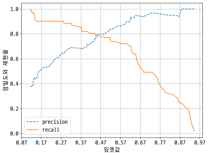
In [27]:
# 정밀도와 재현율의 임곗값에 따른 값 변화를 곡선 형태의 그래프로 시각화
import matplotlib.pyplot as plt
In [28]:
# 그래프로 만들기
def precision_recall_curve_plot(y_test, pred_proba_1):
    from sklearn.metrics import precision_recall_curve
    import matplotlib.pyplot as plt
    # ndarray 추출
    precisions, recalls, thresholds = precision_recall_curve(y_test, pred_proba_1)

    # x축은 threshold, y축은 precision, recall으로 plot 수행. precision은 점선
    plt.figure(figsize=(8, 6))
    threshold_boundary = thresholds.shape[0]
    plt.plot(thresholds, precisions[0:threshold_boundary], linestyle='--', label='precision') # 갯수 맞춰주기
    plt.plot(thresholds, recalls[0:threshold_boundary], label='recall')

    # threshold 값 x축의 scale을 0.1 단위로 변경
    start, end = plt.xlim() # 시작값과 끝값 리던
    plt.xticks(np.round(np.arange(start, end, 0.1), 2))

    # x축, y축 label과 legend, grid설정
    plt.xlabel('임곗값')
    plt.ylabel('정밀도와 재현율')
    plt.legend()
    plt.grid()
    plt.show()
In [29]:
precision_recall_curve_plot(y_test, pred_proba_1)
Out [29]:
정밀도와 재현율의 맹점
업무 환경에 맞게 두 개의 수치를 상호 보완할 수 있는 수준에서 적용돼야 한다.
그렇지 않고 단순히 하나의 성능 지표 수치를 높이기 위한 수단으로 사용돼서는 안된다.
F1 Score
정밀도와 재현율이 어느 한쪽으로 치우치지 않는 수치를 나타낼 때 상대적으로 높은 값을 가진다.
\[F1 = \frac{2}{\frac{1}{recall}+\frac{1}{precision}} = 2*\frac{precision*recall}{precision+recall}\]
In [30]:
from sklearn.metrics import f1_score
In [31]:
f1_score(y_test, pred)
Out [31]:
0.7966101694915254
In [32]:
def get_clf_eval(y_test, pred):
    from sklearn.metrics import accuracy_score, precision_score, recall_score, confusion_matrix, f1_score
    confusion = confusion_matrix(y_test, pred)
    accuracy = accuracy_score(y_test, pred)
    precision = precision_score(y_test, pred)
    recall = recall_score(y_test, pred)
    f1 = f1_score(y_test, pred)
    print('==오차 행렬==')
    print(confusion)
    print(f"정확도: {accuracy:.4f}, 정밀도: {precision:.4f}, 재현율: {recall:.4f}, F1: {f1:.4f}")

thresholds = [0.4, 0.45, 0.5, 0.55, 0.6]
def get_eval_by_threshold(y_test, pred_proba_1, thresholds):
    for custom_threshold in thresholds:
        custom_predict = Binarizer(threshold=custom_threshold).fit_transform(pred_proba_1)
        print('==임곗값:', custom_threshold)
        get_clf_eval(y_test, custom_predict)
get_eval_by_threshold(y_test, pred_proba_1, thresholds)
Out [32]:
==임곗값: 0.4
==오차 행렬==
[[97 21]
 [11 50]]
정확도: 0.8212, 정밀도: 0.7042, 재현율: 0.8197, F1: 0.7576
==임곗값: 0.45
==오차 행렬==
[[105  13]
 [ 13  48]]
정확도: 0.8547, 정밀도: 0.7869, 재현율: 0.7869, F1: 0.7869
==임곗값: 0.5
==오차 행렬==
[[108  10]
 [ 14  47]]
정확도: 0.8659, 정밀도: 0.8246, 재현율: 0.7705, F1: 0.7966
==임곗값: 0.55
==오차 행렬==
[[111   7]
 [ 16  45]]
정확도: 0.8715, 정밀도: 0.8654, 재현율: 0.7377, F1: 0.7965
==임곗값: 0.6
==오차 행렬==
[[113   5]
 [ 17  44]]
정확도: 0.8771, 정밀도: 0.8980, 재현율: 0.7213, F1: 0.8000
임곗값이 0.6일 때 F1 스코어가 가장 높지만 재현율이 크게 감소하고 있으니 주의해야 한다.
여러 평가 지표가 있으니 상황과 데이터에 맞게 선택해야 한다!
ROC 곡선과 AUC
ROC곡선의 아래 영역의 면적을 AUC score라 한다.
AUC는 1에 가까울수록 좋다.
- ROC곡선
FPR(False Positive Rate)이 변할 때 TPR(True Positive Rate;재현율;민감도)이 어떻게 변하는지를 나타내는 곡선이다.
TNR(특이성;Specificity) = \(\frac{TN}{FP+TN}\)
FPR(실제 0인 것 중에 못맞춘 것) = \(\frac{FP}{FP+TN} = 1 - TNR = 1- 특이성\)
In [33]:
from sklearn.metrics import roc_curve
In [34]:
fprs, tprs, thresholds = roc_curve(y_test, pred_proba_1) # 1이 될 확률
In [35]:
# 그래프 함수
def roc_curve_plot(y_test, pred_proba_1):
    from sklearn.metrics import roc_curve
    import matplotlib.pyplot as plt
    # 임곗값에 따른 FPR, TPR 값을 반환받음
    fprs, tprs, thresholds = roc_curve(y_test, pred_proba_1)
    # ROC 곡선 그래프
    plt.plot(fprs, tprs, label='ROC')
    # 가운데 대각선 직선
    plt.plot([0, 1], [0,1], 'k--', label='Random') # k--: 검은 점선

    start, end = plt.xlim()
    plt.xticks(np.round(np.arange(start, end, 0.1), 2))
    plt.xlim(0, 1)
    plt.ylim(0, 1)
    plt.xlabel('FPR( 1 - Specificity )')
    plt.ylabel('TRP( Recall )')
    plt.legend()
In [36]:
roc_curve_plot(y_test, pred_proba_1)
Out [36]:
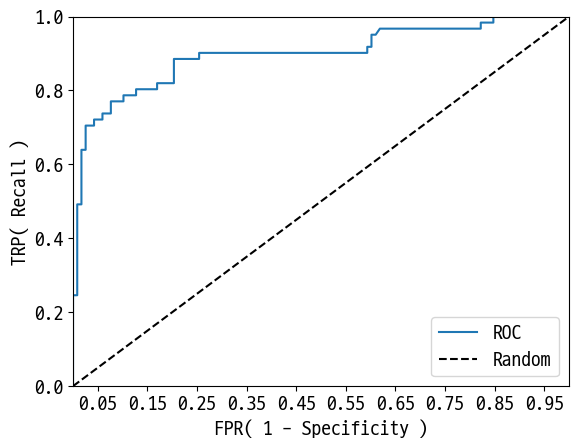
분류의 성능 지표로 사용되는 것은 ROC 곡선 면적에 기반한 AUC값으로 결정한다.
일반적으로 1에 가까울수록 좋은 수치이다.
In [37]:
from sklearn.metrics import roc_auc_score
In [38]:
roc_auc_score(y_test, pred_proba_1)
Out [38]:
0.8986524034454015
In [39]:
# 최종 완성된 평가 함수
def get_clf_eval(y_test, pred, pred_proba_1):
    from sklearn.metrics import accuracy_score, precision_score, recall_score, confusion_matrix, f1_score, roc_auc_score
    confusion = confusion_matrix(y_test, pred)
    accuracy = accuracy_score(y_test, pred)
    precision = precision_score(y_test, pred)
    recall = recall_score(y_test, pred)
    f1 = f1_score(y_test, pred)
    auc = roc_auc_score(y_test, pred_proba_1)
    print('==오차 행렬==')
    print(confusion)
    print(f"정확도: {accuracy:.4f}, 정밀도: {precision:.4f}, 재현율: {recall:.4f}, F1: {f1:.4f}, AUC: {auc:.4f}")
Reference
- 이 포스트는 SeSAC 인공지능 자연어처리, 컴퓨터비전 기술을 활용한 응용 SW 개발자 양성 과정 - 심선조 강사님의 강의를 정리한 내용입니다.
댓글남기기