
Machine Learning (7) - 분류 / 피마 인디언 당뇨병 예측
평가
피마 인디언 당뇨병 예측
고립된 지역에서 혈통이 지속돼 왔으나 20세기 후반에 서구화된 식습관으로 많은 당뇨환자가 발생했다.
따라서 당뇨의 원인중 하나인 유전적 특성을 배제하고 후천적 환경요인(식습관)과 당뇨병의 연관성에 대해 연구가 가능했다.
In [1]:
import numpy as np
import pandas as pd
import matplotlib.pyplot as plt
from sklearn.model_selection import train_test_split
from sklearn.preprocessing import StandardScaler
from sklearn.linear_model import LogisticRegression # 회귀모델을 이진분류용으로 사용
In [2]:
df = pd.read_csv('diabetes.csv')
df.sample(3)
Out [2]:
| Pregnancies | Glucose | BloodPressure | SkinThickness | Insulin | BMI | DiabetesPedigreeFunction | Age | Outcome | |
|---|---|---|---|---|---|---|---|---|---|
| 604 | 4 | 183 | 0 | 0 | 0 | 28.4 | 0.212 | 36 | 1 |
| 699 | 4 | 118 | 70 | 0 | 0 | 44.5 | 0.904 | 26 | 0 |
| 107 | 4 | 144 | 58 | 28 | 140 | 29.5 | 0.287 | 37 | 0 |
데이터 확인
In [3]:
df.info() # null 없음, 모두 숫자값
Out [3]:
<class 'pandas.core.frame.DataFrame'>
RangeIndex: 768 entries, 0 to 767
Data columns (total 9 columns):
 #   Column                    Non-Null Count  Dtype
---  ------                    --------------  -----
 0   Pregnancies               768 non-null    int64
 1   Glucose                   768 non-null    int64
 2   BloodPressure             768 non-null    int64
 3   SkinThickness             768 non-null    int64
 4   Insulin                   768 non-null    int64
 5   BMI                       768 non-null    float64
 6   DiabetesPedigreeFunction  768 non-null    float64
 7   Age                       768 non-null    int64
 8   Outcome                   768 non-null    int64
dtypes: float64(2), int64(7)
memory usage: 54.1 KB
In [4]:
# 이진분류 레이블 확인
df.Outcome.value_counts()
Out [4]:
0    500
1    268
Name: Outcome, dtype: int64
정밀도, 재현율 곡선 그리기
In [5]:
# X = df.iloc[:, :-1]
# y = df.iloc[;, -1]
X = df.drop(columns=['Outcome'])
y = df['Outcome']
In [6]:
X_train, X_test, y_train, y_test = train_test_split(X, y, test_size=0.2, random_state=156, stratify=y) # stratify: stratified KFold처럼 레이블 비율을 비슷하게 나눔

# 로지스틱 회귀로 학습, 예측, 평가
lr_clf = LogisticRegression(solver='liblinear')
lr_clf.fit(X_train, y_train)
pred = lr_clf.predict(X_test)
pred_proba = lr_clf.predict_proba(X_test)[:, 1] # 1이 될 확룰
In [7]:
# 최종 완성된 평가 함수
def get_clf_eval(y_test, pred, pred_proba_1):
    from sklearn.metrics import accuracy_score, precision_score, recall_score, confusion_matrix, f1_score, roc_auc_score
    confusion = confusion_matrix(y_test, pred)
    accuracy = accuracy_score(y_test, pred)
    precision = precision_score(y_test, pred)
    recall = recall_score(y_test, pred)
    f1 = f1_score(y_test, pred)
    auc = roc_auc_score(y_test, pred_proba_1)
    print('==오차 행렬==')
    print(confusion)
    print(f"정확도: {accuracy:.4f}, 정밀도: {precision:.4f}, 재현율: {recall:.4f}, F1: {f1:.4f}, AUC: {auc:.4f}")

# 그래프로 만들기
def precision_recall_curve_plot(y_test, pred_proba_1):
    from sklearn.metrics import precision_recall_curve
    import matplotlib.pyplot as plt
    # ndarray 추출
    precisions, recalls, thresholds = precision_recall_curve(y_test, pred_proba_1)

    # x축은 threshold, y축은 precision, recall으로 plot 수행. precision은 점선
    plt.figure(figsize=(8, 6))
    threshold_boundary = thresholds.shape[0]
    plt.plot(thresholds, precisions[0:threshold_boundary], linestyle='--', label='precision') # 갯수 맞춰주기
    plt.plot(thresholds, recalls[0:threshold_boundary], label='recall')

    # threshold 값 x축의 scale을 0.1 단위로 변경
    start, end = plt.xlim() # 시작값과 끝값 리던
    plt.xticks(np.round(np.arange(start, end, 0.1), 2))

    # x축, y축 label과 legend, grid설정
    plt.xlabel('임곗값')
    plt.ylabel('정밀도와 재현율')
    plt.legend()
    plt.grid()
    plt.show()
In [8]:
get_clf_eval(y_test, pred, pred_proba)
Out [8]:
==오차 행렬==
[[87 13]
 [22 32]]
정확도: 0.7727, 정밀도: 0.7111, 재현율: 0.5926, F1: 0.6465, AUC: 0.8083
- 낮은 재현율을 좀 더 올려보자!
In [9]:
precision_recall_curve_plot(y_test, pred_proba)
Out [9]:
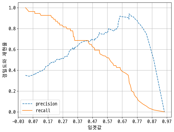
임곗값 0.42정도에 서로 만난다.
하지만 그 지점에서의 정밀도와 재현율이 너무 낮다.
전처리가 제대로 되었는지 확인한다.
전처리 확인
In [10]:
df.describe()
Out [10]:
| Pregnancies | Glucose | BloodPressure | SkinThickness | Insulin | BMI | DiabetesPedigreeFunction | Age | Outcome | |
|---|---|---|---|---|---|---|---|---|---|
| count | 768.000000 | 768.000000 | 768.000000 | 768.000000 | 768.000000 | 768.000000 | 768.000000 | 768.000000 | 768.000000 |
| mean | 3.845052 | 120.894531 | 69.105469 | 20.536458 | 79.799479 | 31.992578 | 0.471876 | 33.240885 | 0.348958 |
| std | 3.369578 | 31.972618 | 19.355807 | 15.952218 | 115.244002 | 7.884160 | 0.331329 | 11.760232 | 0.476951 |
| min | 0.000000 | 0.000000 | 0.000000 | 0.000000 | 0.000000 | 0.000000 | 0.078000 | 21.000000 | 0.000000 |
| 25% | 1.000000 | 99.000000 | 62.000000 | 0.000000 | 0.000000 | 27.300000 | 0.243750 | 24.000000 | 0.000000 |
| 50% | 3.000000 | 117.000000 | 72.000000 | 23.000000 | 30.500000 | 32.000000 | 0.372500 | 29.000000 | 0.000000 |
| 75% | 6.000000 | 140.250000 | 80.000000 | 32.000000 | 127.250000 | 36.600000 | 0.626250 | 41.000000 | 1.000000 |
| max | 17.000000 | 199.000000 | 122.000000 | 99.000000 | 846.000000 | 67.100000 | 2.420000 | 81.000000 | 1.000000 |
min() 값이 0으로 돼 있는 피처가 상당히 많다.(특히 glucose와 bloodpressure 등 0이 나올 수 없는 데이터들이 있다.)
In [11]:
plt.hist(df.Glucose, bins=100)
plt.show()
Out [11]:
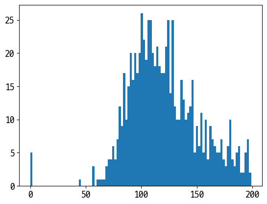
0값이 5개 존재!
In [12]:
df.columns
Out [12]:
Index(['Pregnancies', 'Glucose', 'BloodPressure', 'SkinThickness', 'Insulin',
       'BMI', 'DiabetesPedigreeFunction', 'Age', 'Outcome'],
      dtype='object')
In [13]:
# 0값을 검사할 피처명 리스트
zero_features = ['Glucose', 'BloodPressure', 'SkinThickness', 'Insulin', 'BMI']

# 전체 데이터 건수
total_count = df.Glucose.count()

# feature별로 반복하면서 데이터 값이 0인 데이터 건수를 추출, 퍼센트 계산
for feature in zero_features:
    zero_count = df[df[feature] == 0][feature].count()
    print(f"{feature} 0 건수: {zero_count}건, 퍼센트: {zero_count/total_count*100:.2f}%")
Out [13]:
Glucose 0 건수: 5건, 퍼센트: 0.65%
BloodPressure 0 건수: 35건, 퍼센트: 4.56%
SkinThickness 0 건수: 227건, 퍼센트: 29.56%
Insulin 0 건수: 374건, 퍼센트: 48.70%
BMI 0 건수: 11건, 퍼센트: 1.43%
In [14]:
# zero_features 리스트 내부에 저장된 개별 피처들에 대해서 0값을 평균 값으로 대체
mean_zero_features = df[zero_features].mean()
In [15]:
df[zero_features] = df[zero_features].replace(0, mean_zero_features)
In [16]:
# feature별로 반복하면서 데이터 값이 0인 데이터 건수를 추출, 퍼센트 계산
for feature in zero_features:
    zero_count = df[df[feature] == 0][feature].count()
    print(f"{feature} 0 건수: {zero_count}건, 퍼센트: {zero_count/total_count*100:.2f}%")
Out [16]:
Glucose 0 건수: 0건, 퍼센트: 0.00%
BloodPressure 0 건수: 0건, 퍼센트: 0.00%
SkinThickness 0 건수: 0건, 퍼센트: 0.00%
Insulin 0 건수: 0건, 퍼센트: 0.00%
BMI 0 건수: 0건, 퍼센트: 0.00%
In [17]:
X = df.drop(columns=['Outcome'])
y = df['Outcome']

# StanderdScaler 적용 - 평균0, 분산1(가우시안 정규분포)
scaler = StandardScaler()
X_scaled = scaler.fit_transform(X)

X_train, X_test, y_train, y_test = train_test_split(X_scaled, y, test_size=0.2, random_state=156, stratify=y)

# 로지스틱 회귀로 학습, 예측, 평가
lr_clf = LogisticRegression(solver='liblinear')
lr_clf.fit(X_train, y_train)
pred = lr_clf.predict(X_test)
pred_proba = lr_clf.predict_proba(X_test)[:, 1]

get_clf_eval(y_test, pred, pred_proba)

# ==오차 행렬==
# [[87 13]
#  [22 32]]
# 정확도: 0.7727, 정밀도: 0.7111, 재현율: 0.5926, F1: 0.6465, AUC: 0.8083
Out [17]:
==오차 행렬==
[[90 10]
 [21 33]]
정확도: 0.7987, 정밀도: 0.7674, 재현율: 0.6111, F1: 0.6804, AUC: 0.8433
임곗값을 조절
In [18]:
thresholds = [0.3, 0.33, 0.36, 0.39, 0.42, 0.45, 0.48, 0.5] # 재현율을 높이기 위해 0.5보다 낮은 수치로만 설정
def get_eval_by_threshold(y_test, pred_proba_1, thresholds):
    from sklearn.preprocessing import Binarizer
    for custom_threshold in thresholds:
        custom_predict = Binarizer(threshold=custom_threshold).fit_transform(pred_proba_1.reshape(-1, 1))
        print('==임곗값:', custom_threshold)
        get_clf_eval(y_test, custom_predict, pred_proba_1)
get_eval_by_threshold(y_test, pred_proba, thresholds)
Out [18]:
==임곗값: 0.3
==오차 행렬==
[[65 35]
 [11 43]]
정확도: 0.7013, 정밀도: 0.5513, 재현율: 0.7963, F1: 0.6515, AUC: 0.8433
==임곗값: 0.33
==오차 행렬==
[[71 29]
 [11 43]]
정확도: 0.7403, 정밀도: 0.5972, 재현율: 0.7963, F1: 0.6825, AUC: 0.8433
==임곗값: 0.36
==오차 행렬==
[[76 24]
 [15 39]]
정확도: 0.7468, 정밀도: 0.6190, 재현율: 0.7222, F1: 0.6667, AUC: 0.8433
==임곗값: 0.39
==오차 행렬==
[[78 22]
 [16 38]]
정확도: 0.7532, 정밀도: 0.6333, 재현율: 0.7037, F1: 0.6667, AUC: 0.8433
==임곗값: 0.42
==오차 행렬==
[[84 16]
 [18 36]]
정확도: 0.7792, 정밀도: 0.6923, 재현율: 0.6667, F1: 0.6792, AUC: 0.8433
==임곗값: 0.45
==오차 행렬==
[[85 15]
 [18 36]]
정확도: 0.7857, 정밀도: 0.7059, 재현율: 0.6667, F1: 0.6857, AUC: 0.8433
==임곗값: 0.48
==오차 행렬==
[[88 12]
 [19 35]]
정확도: 0.7987, 정밀도: 0.7447, 재현율: 0.6481, F1: 0.6931, AUC: 0.8433
==임곗값: 0.5
==오차 행렬==
[[90 10]
 [21 33]]
정확도: 0.7987, 정밀도: 0.7674, 재현율: 0.6111, F1: 0.6804, AUC: 0.8433
==임곗값: 0.48
==오차 행렬==
[[88 12]
[19 35]]
정확도: 0.7987, 정밀도: 0.7447, 재현율: 0.6481, F1: 0.6931, AUC: 0.8433
Reference
- 이 포스트는 SeSAC 인공지능 자연어처리, 컴퓨터비전 기술을 활용한 응용 SW 개발자 양성 과정 - 심선조 강사님의 강의를 정리한 내용입니다.
댓글남기기