
Machine Learning (12) - 분류 / 산탄데르 고객 만족 예측
분류
분류 실습 - 캐글 산탄데르 고객 만족 예측
은행의 고객관련 정보로 고객 만족 여부를 예측
데이터 전처리
In [1]:
import numpy as np
import pandas as pd
import matplotlib.pyplot as plt
import warnings
warnings.filterwarnings('ignore')
In [2]:
df = pd.read_csv('santander.csv')
In [3]:
df.info()
Out [3]:
<class 'pandas.core.frame.DataFrame'>
RangeIndex: 76020 entries, 0 to 76019
Columns: 371 entries, ID to TARGET
dtypes: float64(111), int64(260)
memory usage: 215.2 MB
In [4]:
df['TARGET'].value_counts()
Out [4]:
0    73012
1     3008
Name: TARGET, dtype: int64
In [5]:
un_cnt = df[df['TARGET'] == 1].TARGET.count()
total_cnt = df.TARGET.count()
print('불만족 고객 비율:', un_cnt / total_cnt)
Out [5]:
불만족 고객 비율: 0.0395685345961589
In [6]:
df.describe()
Out [6]:
| ID | var3 | var15 | imp_ent_var16_ult1 | imp_op_var39_comer_ult1 | imp_op_var39_comer_ult3 | imp_op_var40_comer_ult1 | imp_op_var40_comer_ult3 | imp_op_var40_efect_ult1 | imp_op_var40_efect_ult3 | ... | saldo_medio_var33_hace2 | saldo_medio_var33_hace3 | saldo_medio_var33_ult1 | saldo_medio_var33_ult3 | saldo_medio_var44_hace2 | saldo_medio_var44_hace3 | saldo_medio_var44_ult1 | saldo_medio_var44_ult3 | var38 | TARGET | |
|---|---|---|---|---|---|---|---|---|---|---|---|---|---|---|---|---|---|---|---|---|---|
| count | 76020.000000 | 76020.000000 | 76020.000000 | 76020.000000 | 76020.000000 | 76020.000000 | 76020.000000 | 76020.000000 | 76020.000000 | 76020.000000 | ... | 76020.000000 | 76020.000000 | 76020.000000 | 76020.000000 | 76020.000000 | 76020.000000 | 76020.000000 | 76020.000000 | 7.602000e+04 | 76020.000000 |
| mean | 75964.050723 | -1523.199277 | 33.212865 | 86.208265 | 72.363067 | 119.529632 | 3.559130 | 6.472698 | 0.412946 | 0.567352 | ... | 7.935824 | 1.365146 | 12.215580 | 8.784074 | 31.505324 | 1.858575 | 76.026165 | 56.614351 | 1.172358e+05 | 0.039569 |
| std | 43781.947379 | 39033.462364 | 12.956486 | 1614.757313 | 339.315831 | 546.266294 | 93.155749 | 153.737066 | 30.604864 | 36.513513 | ... | 455.887218 | 113.959637 | 783.207399 | 538.439211 | 2013.125393 | 147.786584 | 4040.337842 | 2852.579397 | 1.826646e+05 | 0.194945 |
| min | 1.000000 | -999999.000000 | 5.000000 | 0.000000 | 0.000000 | 0.000000 | 0.000000 | 0.000000 | 0.000000 | 0.000000 | ... | 0.000000 | 0.000000 | 0.000000 | 0.000000 | 0.000000 | 0.000000 | 0.000000 | 0.000000 | 5.163750e+03 | 0.000000 |
| 25% | 38104.750000 | 2.000000 | 23.000000 | 0.000000 | 0.000000 | 0.000000 | 0.000000 | 0.000000 | 0.000000 | 0.000000 | ... | 0.000000 | 0.000000 | 0.000000 | 0.000000 | 0.000000 | 0.000000 | 0.000000 | 0.000000 | 6.787061e+04 | 0.000000 |
| 50% | 76043.000000 | 2.000000 | 28.000000 | 0.000000 | 0.000000 | 0.000000 | 0.000000 | 0.000000 | 0.000000 | 0.000000 | ... | 0.000000 | 0.000000 | 0.000000 | 0.000000 | 0.000000 | 0.000000 | 0.000000 | 0.000000 | 1.064092e+05 | 0.000000 |
| 75% | 113748.750000 | 2.000000 | 40.000000 | 0.000000 | 0.000000 | 0.000000 | 0.000000 | 0.000000 | 0.000000 | 0.000000 | ... | 0.000000 | 0.000000 | 0.000000 | 0.000000 | 0.000000 | 0.000000 | 0.000000 | 0.000000 | 1.187563e+05 | 0.000000 |
| max | 151838.000000 | 238.000000 | 105.000000 | 210000.000000 | 12888.030000 | 21024.810000 | 8237.820000 | 11073.570000 | 6600.000000 | 6600.000000 | ... | 50003.880000 | 20385.720000 | 138831.630000 | 91778.730000 | 438329.220000 | 24650.010000 | 681462.900000 | 397884.300000 | 2.203474e+07 | 1.000000 |
8 rows × 371 columns
In [7]:
# 최솟값 -999999을 최빈값 2로 수정
df['var3'].replace(-999999, 2, inplace=True)
df.drop(columns=['ID'], inplace=True)
In [8]:
df.describe()
Out [8]:
| var3 | var15 | imp_ent_var16_ult1 | imp_op_var39_comer_ult1 | imp_op_var39_comer_ult3 | imp_op_var40_comer_ult1 | imp_op_var40_comer_ult3 | imp_op_var40_efect_ult1 | imp_op_var40_efect_ult3 | imp_op_var40_ult1 | ... | saldo_medio_var33_hace2 | saldo_medio_var33_hace3 | saldo_medio_var33_ult1 | saldo_medio_var33_ult3 | saldo_medio_var44_hace2 | saldo_medio_var44_hace3 | saldo_medio_var44_ult1 | saldo_medio_var44_ult3 | var38 | TARGET | |
|---|---|---|---|---|---|---|---|---|---|---|---|---|---|---|---|---|---|---|---|---|---|
| count | 76020.000000 | 76020.000000 | 76020.000000 | 76020.000000 | 76020.000000 | 76020.000000 | 76020.000000 | 76020.000000 | 76020.000000 | 76020.000000 | ... | 76020.000000 | 76020.000000 | 76020.000000 | 76020.000000 | 76020.000000 | 76020.000000 | 76020.000000 | 76020.000000 | 7.602000e+04 | 76020.000000 |
| mean | 2.716483 | 33.212865 | 86.208265 | 72.363067 | 119.529632 | 3.559130 | 6.472698 | 0.412946 | 0.567352 | 3.160715 | ... | 7.935824 | 1.365146 | 12.215580 | 8.784074 | 31.505324 | 1.858575 | 76.026165 | 56.614351 | 1.172358e+05 | 0.039569 |
| std | 9.447971 | 12.956486 | 1614.757313 | 339.315831 | 546.266294 | 93.155749 | 153.737066 | 30.604864 | 36.513513 | 95.268204 | ... | 455.887218 | 113.959637 | 783.207399 | 538.439211 | 2013.125393 | 147.786584 | 4040.337842 | 2852.579397 | 1.826646e+05 | 0.194945 |
| min | 0.000000 | 5.000000 | 0.000000 | 0.000000 | 0.000000 | 0.000000 | 0.000000 | 0.000000 | 0.000000 | 0.000000 | ... | 0.000000 | 0.000000 | 0.000000 | 0.000000 | 0.000000 | 0.000000 | 0.000000 | 0.000000 | 5.163750e+03 | 0.000000 |
| 25% | 2.000000 | 23.000000 | 0.000000 | 0.000000 | 0.000000 | 0.000000 | 0.000000 | 0.000000 | 0.000000 | 0.000000 | ... | 0.000000 | 0.000000 | 0.000000 | 0.000000 | 0.000000 | 0.000000 | 0.000000 | 0.000000 | 6.787061e+04 | 0.000000 |
| 50% | 2.000000 | 28.000000 | 0.000000 | 0.000000 | 0.000000 | 0.000000 | 0.000000 | 0.000000 | 0.000000 | 0.000000 | ... | 0.000000 | 0.000000 | 0.000000 | 0.000000 | 0.000000 | 0.000000 | 0.000000 | 0.000000 | 1.064092e+05 | 0.000000 |
| 75% | 2.000000 | 40.000000 | 0.000000 | 0.000000 | 0.000000 | 0.000000 | 0.000000 | 0.000000 | 0.000000 | 0.000000 | ... | 0.000000 | 0.000000 | 0.000000 | 0.000000 | 0.000000 | 0.000000 | 0.000000 | 0.000000 | 1.187563e+05 | 0.000000 |
| max | 238.000000 | 105.000000 | 210000.000000 | 12888.030000 | 21024.810000 | 8237.820000 | 11073.570000 | 6600.000000 | 6600.000000 | 8237.820000 | ... | 50003.880000 | 20385.720000 | 138831.630000 | 91778.730000 | 438329.220000 | 24650.010000 | 681462.900000 | 397884.300000 | 2.203474e+07 | 1.000000 |
8 rows × 370 columns
In [9]:
X = df.iloc[:, :-1]
y = df.iloc[:, -1]
In [10]:
from sklearn.model_selection import train_test_split
In [11]:
# 학습/테스트 데이터 분리
X_train, X_test, y_train, y_test = train_test_split(X, y, test_size=0.2, random_state=0)
In [12]:
train_cnt = y_train.count()
test_cnt = y_test.count()
In [13]:
# 학습 데이터 레이블의 비율
y_train.value_counts() / train_cnt
Out [13]:
0    0.960964
1    0.039036
Name: TARGET, dtype: float64
In [14]:
# 테스트 데이터 레이블의 비율
y_test.value_counts() / test_cnt
Out [14]:
0    0.9583
1    0.0417
Name: TARGET, dtype: float64
In [15]:
# 학습/검증 데이터 분리
X_tr, X_val, y_tr, y_val = train_test_split(X_train, y_train, test_size=0.3, random_state=0)
XGBoost 모델 학습과 하이퍼 파라미터 튜닝
In [16]:
from xgboost import XGBClassifier
from sklearn.metrics import roc_auc_score
In [17]:
xgb_clf = XGBClassifier(n_estimators=500, learning_rate=0.05, random_state=156)
xgb_clf.fit(X_tr, y_tr, early_stopping_rounds=100, eval_metric='auc', eval_set=[(X_tr, y_tr), (X_val, y_val)], verbose=False)
Out [17]:
XGBClassifier(base_score=0.5, booster='gbtree', colsample_bylevel=1,
              colsample_bynode=1, colsample_bytree=1, enable_categorical=False,
              gamma=0, gpu_id=-1, importance_type=None,
              interaction_constraints='', learning_rate=0.05, max_delta_step=0,
              max_depth=6, min_child_weight=1, missing=nan,
              monotone_constraints='()', n_estimators=500, n_jobs=8,
              num_parallel_tree=1, predictor='auto', random_state=156,
              reg_alpha=0, reg_lambda=1, scale_pos_weight=1, subsample=1,
              tree_method='exact', validate_parameters=1, verbosity=None)
In [18]:
xgb_roc_score = roc_auc_score(y_test, xgb_clf.predict_proba(X_test)[:, 1])
print('ROC AUC:', xgb_roc_score)
Out [18]:
ROC AUC: 0.842853493090032
In [19]:
from hyperopt import hp
In [20]:
## search space 설정

# max_depth는 5~15 1간격, min_child_weight는 1~6 1간격
# colsample_bytree는 0.5~0.95사이, learning_rate는 0.01~0.2사이 정규 분포된 값
xgb_search_space = {'max_depth': hp.quniform('max_depth', 5, 15, 1),
                    'min_child_weight': hp.quniform('min_child_weight', 1, 6, 1),
                    'colsample_bytree': hp.uniform('colsample_bytree', 0.5, 0.95),
                    'learning_rate': hp.uniform('learning_rate', 0.01, 0.2)
}
In [21]:
from sklearn.model_selection import KFold
from sklearn.metrics import roc_auc_score
In [22]:
## 목적 함수 설정.

# 추후 fmin()에서 입력된 search_space값으로 XGBClassifier 교차 검증 학습 후 -1* roc_auc 평균 값을 반환.
def objective_func(search_space):
    xgb_clf = XGBClassifier(n_estimators=100, max_depth=int(search_space['max_depth']),
                            min_child_weight=int(search_space['min_child_weight']),
                            colsample_bytree=search_space['colsample_bytree'],
                            learning_rate=search_space['learning_rate']
                           )
    # 3개 k-fold 방식으로 평가된 roc_auc 지표를 담는 list
    roc_auc_list= []

    # 3개 k-fold방식 적용
    kf = KFold(n_splits=3)
    # X_train을 다시 학습과 검증용 데이터로 분리
    for tr_index, val_index in kf.split(X_train):
        # kf.split(X_train)으로 추출된 학습과 검증 index값으로 학습과 검증 데이터 세트 분리
        X_tr, y_tr = X_train.iloc[tr_index], y_train.iloc[tr_index]
        X_val, y_val = X_train.iloc[val_index], y_train.iloc[val_index]
        # early stopping은 30회로 설정하고 추출된 학습과 검증 데이터로 XGBClassifier 학습 수행.
        xgb_clf.fit(X_tr, y_tr, early_stopping_rounds=30, eval_metric='auc',
                   eval_set=[(X_tr, y_tr), (X_val, y_val)], verbose=False)

        # 1로 예측한 확률값 추출후 roc auc 계산하고 평균 roc auc 계산을 위해 list에 결과값 담음.
        score = roc_auc_score(y_val, xgb_clf.predict_proba(X_val)[:, 1])
        roc_auc_list.append(score)

    # 3개 k-fold로 계산된 roc_auc값의 평균값을 반환하되,
    # HyperOpt는 목적함수의 최소값을 위한 입력값을 찾으므로 -1을 곱한 뒤 반환.
    return -1 * np.mean(roc_auc_list)
In [23]:
from hyperopt import fmin, tpe, Trials
In [24]:
trials = Trials() #30분 이상 소요

# fmin()함수를 호출. max_evals지정된 횟수만큼 반복 후 목적함수의 최소값을 가지는 최적 입력값 추출.
best = fmin(fn=objective_func,
            space=xgb_search_space,
            algo=tpe.suggest,
            max_evals=50, # 최대 반복 횟수를 지정합니다.
            trials=trials, rstate=np.random.default_rng(seed=30))

print('best:', best)
Out [24]:
100%|███████████████████████████████████████████████| 50/50 [23:41<00:00, 28.44s/trial, best loss: -0.8377636283109627]
best: {'colsample_bytree': 0.5749934608268169, 'learning_rate': 0.15145639274819528, 'max_depth': 5.0, 'min_child_weight': 6.0}
In [25]:
# n_estimators를 500증가 후 최적으로 찾은 하이퍼 파라미터를 기반으로 학습과 예측 수행.
xgb_clf = XGBClassifier(n_estimators=500, learning_rate=round(best['learning_rate'], 5),
                        max_depth=int(best['max_depth']), min_child_weight=int(best['min_child_weight']),
                        colsample_bytree=round(best['colsample_bytree'], 5)
                       )

# evaluation metric을 auc로, early stopping은 100 으로 설정하고 학습 수행.
xgb_clf.fit(X_tr, y_tr, early_stopping_rounds=100,
            eval_metric="auc",eval_set=[(X_tr, y_tr), (X_val, y_val)], verbose=False)

xgb_roc_score = roc_auc_score(y_test, xgb_clf.predict_proba(X_test)[:,1])
print('ROC AUC: {0:.4f}'.format(xgb_roc_score))
Out [25]:
ROC AUC: 0.8457
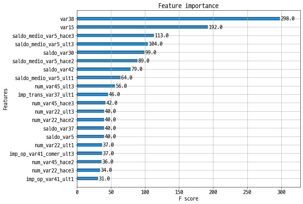
In [26]:
from xgboost import plot_importance
import matplotlib.pyplot as plt
%matplotlib inline

fig, ax = plt.subplots(1,1,figsize=(10,8))
plot_importance(xgb_clf, ax=ax , max_num_features=20,height=0.4)
Out [26]:
<AxesSubplot:title={'center':'Feature importance'}, xlabel='F score', ylabel='Features'>
LightGBM 모델 학습과 하이퍼 파라미터 튜닝
In [27]:
from lightgbm import LGBMClassifier

lgbm_clf = LGBMClassifier(n_estimators=500)

eval_set=[(X_tr, y_tr), (X_val, y_val)]
lgbm_clf.fit(X_tr, y_tr, early_stopping_rounds=100, eval_metric="auc", eval_set=eval_set, verbose=False)

lgbm_roc_score = roc_auc_score(y_test, lgbm_clf.predict_proba(X_test)[:,1])
print('ROC AUC: {0:.4f}'.format(lgbm_roc_score))
Out [27]:
ROC AUC: 0.8384
In [28]:
lgbm_search_space = {'num_leaves': hp.quniform('num_leaves', 32, 64, 1),
                     'max_depth': hp.quniform('max_depth', 100, 160, 1),
                     'min_child_samples': hp.quniform('min_child_samples', 60, 100, 1),
                     'subsample': hp.uniform('subsample', 0.7, 1),
                     'learning_rate': hp.uniform('learning_rate', 0.01, 0.2)
                    }
In [29]:
def objective_func(search_space):
    lgbm_clf =  LGBMClassifier(n_estimators=100, num_leaves=int(search_space['num_leaves']),
                               max_depth=int(search_space['max_depth']),
                               min_child_samples=int(search_space['min_child_samples']),
                               subsample=search_space['subsample'],
                               learning_rate=search_space['learning_rate'])
    # 3개 k-fold 방식으로 평가된 roc_auc 지표를 담는 list
    roc_auc_list = []

    # 3개 k-fold방식 적용
    kf = KFold(n_splits=3)
    # X_train을 다시 학습과 검증용 데이터로 분리
    for tr_index, val_index in kf.split(X_train):
        # kf.split(X_train)으로 추출된 학습과 검증 index값으로 학습과 검증 데이터 세트 분리
        X_tr, y_tr = X_train.iloc[tr_index], y_train.iloc[tr_index]
        X_val, y_val = X_train.iloc[val_index], y_train.iloc[val_index]

        # early stopping은 30회로 설정하고 추출된 학습과 검증 데이터로 XGBClassifier 학습 수행.
        lgbm_clf.fit(X_tr, y_tr, early_stopping_rounds=30, eval_metric="auc",
           eval_set=[(X_tr, y_tr), (X_val, y_val)], verbose=False)

        # 1로 예측한 확률값 추출후 roc auc 계산하고 평균 roc auc 계산을 위해 list에 결과값 담음.
        score = roc_auc_score(y_val, lgbm_clf.predict_proba(X_val)[:, 1])
        roc_auc_list.append(score)

    # 3개 k-fold로 계산된 roc_auc값의 평균값을 반환하되,
    # HyperOpt는 목적함수의 최소값을 위한 입력값을 찾으므로 -1을 곱한 뒤 반환.
    return -1*np.mean(roc_auc_list)
In [30]:
from hyperopt import fmin, tpe, Trials

trials = Trials()

# fmin()함수를 호출. max_evals지정된 횟수만큼 반복 후 목적함수의 최소값을 가지는 최적 입력값 추출.
best = fmin(fn=objective_func, space=lgbm_search_space, algo=tpe.suggest,
            max_evals=50, # 최대 반복 횟수를 지정합니다.
            trials=trials, rstate=np.random.default_rng(seed=30))

print('best:', best)
Out [30]:
100%|███████████████████████████████████████████████| 50/50 [02:37<00:00,  3.16s/trial, best loss: -0.8357657786434084]
best: {'learning_rate': 0.08592271133758617, 'max_depth': 121.0, 'min_child_samples': 69.0, 'num_leaves': 41.0, 'subsample': 0.9148958093027029}
In [31]:
lgbm_clf =  LGBMClassifier(n_estimators=500, num_leaves=int(best['num_leaves']),
                           max_depth=int(best['max_depth']),
                           min_child_samples=int(best['min_child_samples']),
                           subsample=round(best['subsample'], 5),
                           learning_rate=round(best['learning_rate'], 5)
                          )

# evaluation metric을 auc로, early stopping은 100 으로 설정하고 학습 수행.
lgbm_clf.fit(X_tr, y_tr, early_stopping_rounds=100,
            eval_metric="auc",eval_set=[(X_tr, y_tr), (X_val, y_val)], verbose=False)

lgbm_roc_score = roc_auc_score(y_test, lgbm_clf.predict_proba(X_test)[:,1])
print('ROC AUC: {0:.4f}'.format(lgbm_roc_score))
Out [31]:
ROC AUC: 0.8446
Reference
- 이 포스트는 SeSAC 인공지능 자연어처리, 컴퓨터비전 기술을 활용한 응용 SW 개발자 양성 과정 - 심선조 강사님의 강의를 정리한 내용입니다.
댓글남기기