Machine Learning (18) - 차원 축소 / PCA

---

차원 축소

개요

차원 축소는 매우 많은 피처로 구성된 다차원 데이터 세트의 차원을 축소해 새로운 치원의 데이터 세트를 생성하는 것이다.
수백 개 이상의 피처로 구성된 데이터 세트의 경우 상대적으로 적은 차원에서 학습된 모델보다 예측 신뢰도가 떨어진다.
선형 회귀와 같은 선형 모넬에서는 입력 변수 간의 상관관계가 높을 경우 이로 인한 다중 공선성 문제로 모댈의 예측 성능이 저하된다.

일반적으로 차원 축소는 피처 선택(feature selection) 과 피처 추출(feature traction) 로 나눌 수 있다.

• 피처 선택(특성 선택) : 특정 피처에 종속성이 강한 불필요한 피처는 아예 제거하고, 데이터의 특정을 잘 나타내는 주요 피처만 선택
• 피처 추출(특성 추출) : 기존 피처를 저차원의 중요 피처로 압축해서 추출. 이렇게 새롭게 추출된 중요 특성은 기존의 피처가 압축된 것이므로 기존의 피처외는 완전히 다른 값

PCA(Principal Compoennt Analysis)

여러 변수 간에 존재하는 상하관계를 이용해 이를 대표하는 주성분(Principal Component)을 추출해 차원을 축소하는 기법이다.

제일 먼저 가장 큰 데이터 변동성(Variance)을 기반으로 첫 번째 벡터 축을 생성하고, 두 번째 축은 이 벡터 축에 직각이 되는 벡터(직교 벡터)를 축으로 한다.
원본 데이터의 피처 개수에 비해 매우 작은 주성분으로 원본 데이터의 총 변동성을 대부분 설명할 수 있는 분석법이다.

In [1]:

from sklearn.datasets import load_iris
import pandas as pd
import matplotlib.pyplot as plt

In [2]:

iris = load_iris(as_frame=True)
iris.data.head(2)

Out [2]:

	sepal length (cm)	sepal width (cm)	petal length (cm)	petal width (cm)
0	5.1	3.5	1.4	0.2
1	4.9	3.0	1.4	0.2

In [3]:

iris.data.columns = ['sepal_length', 'sepal_width', 'petal_length', 'petal_width']
iris.data.head(2)

Out [3]:

	sepal_length	sepal_width	petal_length	petal_width
0	5.1	3.5	1.4	0.2
1	4.9	3.0	1.4	0.2

In [4]:

iris.data['target'] = iris.target
iris.data.head(2)

Out [4]:

	sepal_length	sepal_width	petal_length	petal_width	target
0	5.1	3.5	1.4	0.2	0
1	4.9	3.0	1.4	0.2	0

In [5]:

df = iris.data

In [6]:

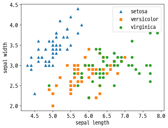
# 세모, 네모, 동그라미
markers=['^', 's', 'o']

for i, marker in enumerate(markers):
    x = df[df['target']==i]['sepal_length']
    y = df[df['target']==i]['sepal_width']
    plt.scatter(x, y, marker=marker, label=iris.target_names[i])
    
plt.legend()
plt.xlabel('sepal length')
plt.ylabel('sepal width')
plt.show()

Out [6]:

In [7]:

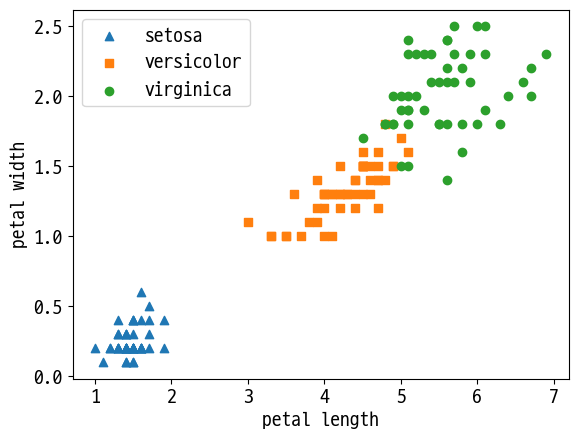
markers=['^', 's', 'o']

for i, marker in enumerate(markers):
    x = df[df['target']==i]['petal_length']
    y = df[df['target']==i]['petal_width']
    plt.scatter(x, y, marker=marker, label=iris.target_names[i])
    
plt.legend()
plt.xlabel('petal length')
plt.ylabel('petal width')
plt.show()

Out [7]:

• PCA 적용 전 스케일링 - StandardScaler

In [8]:

from sklearn.preprocessing import StandardScaler

In [9]:

# target 제외 StandardScaler 적용
df_scaled = StandardScaler().fit_transform(df.iloc[:, :-1])

• PCA적용

In [10]:

from sklearn.decomposition import PCA

In [11]:

pca = PCA(n_components=2) # n_components 줄일 목표값
iris_pca = pca.fit_transform(df_scaled)
print(iris_pca.shape)

Out [11]:

(150, 2)

In [12]:

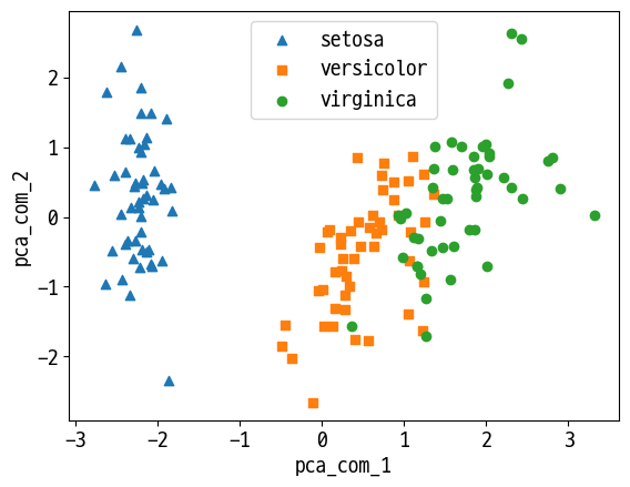
# DataFrame으로 변환
pca_columns = ['pca_com_1', 'pca_com_2']
df_pca = pd.DataFrame(iris_pca, columns=pca_columns)
df_pca['target'] = iris.target
df_pca.head(2)

Out [12]:

	pca_com_1	pca_com_2	target
0	-2.264703	0.480027	0
1	-2.080961	-0.674134	0

In [13]:

markers=['^', 's', 'o']

for i, marker in enumerate(markers):
    x = df_pca[df_pca['target']==i]['pca_com_1']
    y = df_pca[df_pca['target']==i]['pca_com_2']
    plt.scatter(x, y, marker=marker, label=iris.target_names[i])
    
plt.legend()
plt.xlabel('pca_com_1')
plt.ylabel('pca_com_2')
plt.show()

Out [13]:

In [14]:

# component 별 원본 데이터의 변동성 확인
pca.explained_variance_ratio_

Out [14]:

array([0.72962445, 0.22850762])

• 모델 적용 후 결과 확인

In [15]:

from sklearn.ensemble import RandomForestClassifier
from sklearn.model_selection import cross_val_score
import numpy as np

In [16]:

rf_clf = RandomForestClassifier(random_state=156)
# 원본 데이터로 학습/예측/평가
scores = cross_val_score(rf_clf, iris.data.iloc[:, :-1], iris.target, scoring='accuracy', cv=3)
print('PCA 변환 데이터 교차 검증 개별 정확도:', scores)
print('PCA 변환 데이터 평균 정확도:', np.mean(scores))

Out [16]:

PCA 변환 데이터 교차 검증 개별 정확도: [0.98 0.94 0.96]
PCA 변환 데이터 평균 정확도: 0.96

In [17]:

# 변환 데이터로 학습/예측/평가
scores = cross_val_score(rf_clf, df_pca.iloc[:, :-1], iris.target, scoring='accuracy', cv=3)
print('PCA 변환 데이터 교차 검증 개별 정확도:', scores)
print('PCA 변환 데이터 평균 정확도:', np.mean(scores))

Out [17]:

PCA 변환 데이터 교차 검증 개별 정확도: [0.88 0.88 0.88]
PCA 변환 데이터 평균 정확도: 0.88

Reference

• 이 포스트는 SeSAC 인공지능 자연어처리, 컴퓨터비전 기술을 활용한 응용 SW 개발자 양성 과정 - 심선조 강사님의 강의를 정리한 내용입니다.