음성 처리 - 사운드 툴

2023년 01월 30일 3 분 소요

Sound Tools

IPython.ipd

사운드 파일 재생

In [1]:

import numpy as np
import IPython.display as ipd

In [2]:

sr = 16000 # 샘플링 레이트
T = 2.0
amp = 1.0 # 진폭
f = 440 # 440Hz

t = np.linspace(0, T, int(T*sr))
y = amp * np.sin(2.0*np.pi*f*t)

ipd.Audio(y, rate=sr)

Out [2]:

TTS는 seq2seq와 구조가 유사하다.

악기 합성

In [3]:

pitch_do = 523.25
pitch_re = 587.32
pitch_mi = 659.25
pitch_pa = 698.45
pitch_sol = 783.99
pitch_la = 880.0
pitch_si = 987.76
pitch_do2 = 1046.5

In [4]:

# 음 하나만
f = pitch_pa
y = amp * np.sin(2.0*np.pi*f*t)

ipd.Audio(y, rate=sr)

Out [4]:

In [5]:

# C major chord 합성
note_root = amp * np.sin(2.0*np.pi*pitch_do*t) # 근음(기초음)
note_3rd = amp * np.sin(2.0*np.pi*pitch_mi*t)
note_5th = amp * np.sin(2.0*np.pi*pitch_sol*t)

C_major_chord = note_root + note_3rd + note_5th
ipd.Audio(C_major_chord, rate=sr)

Out [5]:

In [6]:

pitch_miplat = 622.25

# C minor chord 합성
note_root = amp * np.sin(2.0*np.pi*pitch_do*t)
note_3rd = amp * np.sin(2.0*np.pi*pitch_miplat*t)
note_5th = amp * np.sin(2.0*np.pi*pitch_sol*t)

C_minor_chord = note_root + note_3rd + note_5th
ipd.Audio(C_minor_chord, rate=sr)

Out [6]:

root가 아니라 구성요소(배음)를 찾는게 중요! -> 소리의 온도
음성인식에서 목소리의 지문 역할을 한다.

노래 합성

In [7]:

# 파형 위로 쌓기
np1 = np.array([1,2,3])
np2 = np.array([4,5,6])
np1+np2

Out [7]:

array([5, 7, 9])

In [8]:

# 파형 옆으로 쌓기
np12 = np.append(np1, np2)
np12

Out [8]:

array([1, 2, 3, 4, 5, 6])

In [9]:

# 솔솔 라라 솔솔미 솔솔미미레
# 위의 위로 쌓기와 다른 옆으로 쌓기

In [10]:

pitch_0 = 0
# 0.5초짜리 음표 생성
T = 0.5
t = np.linspace(0, T, int(T*sr))
note_do = amp * np.sin(2.0*np.pi*pitch_do*t)
note_re = amp * np.sin(2.0*np.pi*pitch_re*t)
note_mi = amp * np.sin(2.0*np.pi*pitch_mi*t)
note_pa = amp * np.sin(2.0*np.pi*pitch_pa*t)
note_sol = amp * np.sin(2.0*np.pi*pitch_sol*t)
note_la = amp * np.sin(2.0*np.pi*pitch_la*t)
note_si = amp * np.sin(2.0*np.pi*pitch_si*t)
note_do2 = amp * np.sin(2.0*np.pi*pitch_do2*t)
note_0 = amp * np.sin(2.0*np.pi*pitch_0*t)

sb = [note_sol, note_sol, note_la, note_la, note_sol, note_sol, note_mi, note_0, note_sol, note_sol, note_mi, note_mi, note_re, note_0]
school_bell = np.array([])
for i in sb:
    school_bell = np.append(school_bell, i)

# school_bell = note_sol
# school_bell = np.append(school_bell, note_sol)
# school_bell = np.append(school_bell, note_la)
# school_bell = np.append(school_bell, note_la)
# school_bell = np.append(school_bell, note_sol)
# school_bell = np.append(school_bell, note_sol)
# school_bell = np.append(school_bell, note_mi)
ipd.Audio(school_bell, rate=sr)

Out [10]:

In [11]:

def make_song(string):
    syllable = {'도':note_do, '레':note_re, '미':note_mi, '파':note_pa, '솔':note_sol, '라':note_la, '시':note_si, ' ':note_0}
    song = np.array([])
    for note in string:
        song = np.append(song, syllable[note])
    return ipd.Audio(song, rate=sr)

In [12]:

make_song('미미레도레미 미 미')

Out [12]:

In [13]:

make_song('라라 라시라 라 라라 라라 라 라 라솔 솔라 라솔미미 라솔라솔라 라솔미미 라 라 라시라 라 라라 라솔 솔라솔 솔라 라솔미미')

Out [13]:

In [14]:

make_song('라라라라라 시 라라 솔라라')

Out [14]:

soundfile

사운드 파일 저장, 불러오기

In [15]:

# !pip install soundfile

In [16]:

import soundfile
soundfile.write('학교종이땡땡땡.wav', school_bell, sr, format='WAV')

In [17]:

sound_contents, file_sampling_rate = soundfile.read('학교종이땡땡땡.wav')

In [18]:

ipd.Audio(sound_contents, rate=sr)

Out [18]:

librosa

In [19]:

# !pip install librosa

In [20]:

import matplotlib.pyplot as plt
import librosa.display

In [21]:

librosa.__version__

Out [21]:

'0.9.2'

In [22]:

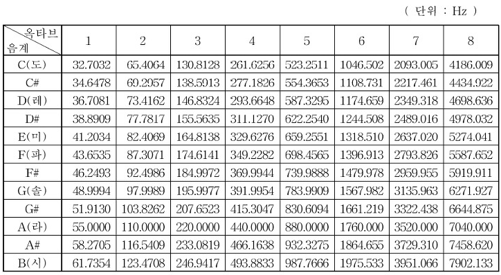
plt.figure(figsize=(14, 5))
librosa.display.waveshow(sound_contents, sr=file_sampling_rate)
plt.show()

Out [22]:

In [23]:

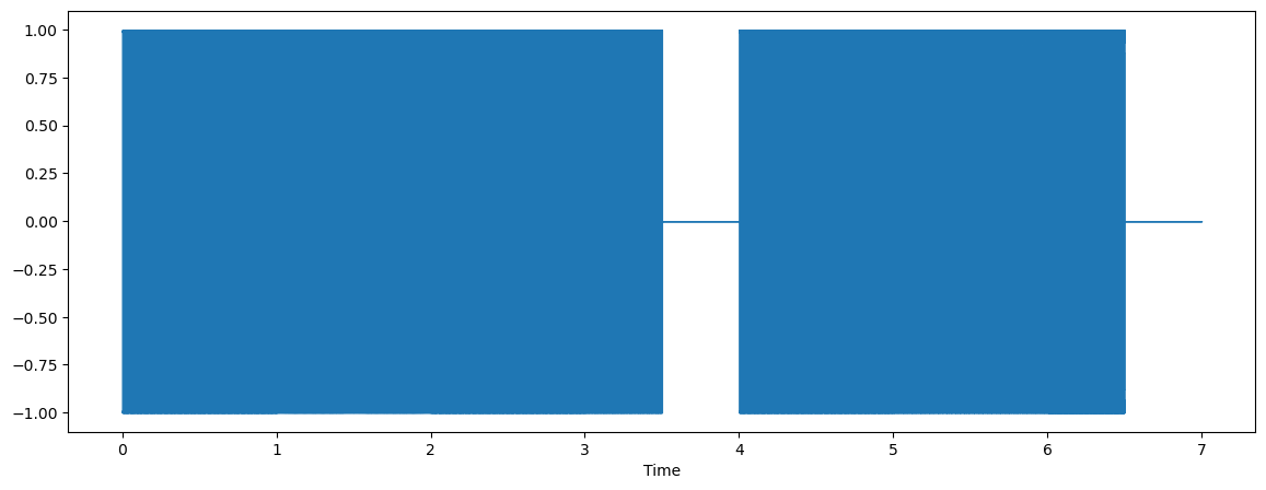
plt.figure(figsize=(14, 5))
librosa.display.waveshow(sound_contents[:100], sr=file_sampling_rate)
plt.show()

Out [23]:

양자화 효과때문에 끊어져 보임

한 주기만 계산해 보여주기

In [24]:

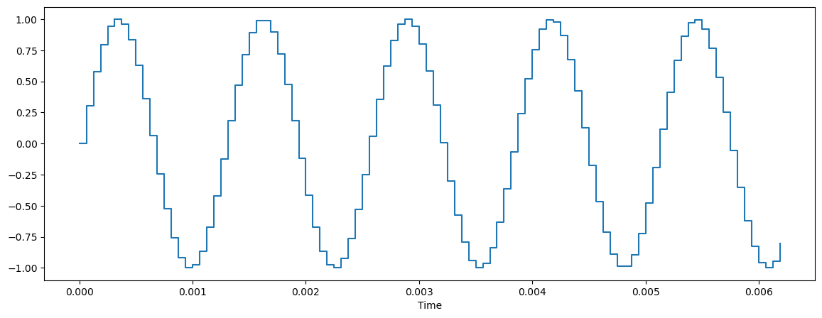
a_cycle_time = int(file_sampling_rate/pitch_sol)+1 # 1초를 구성하는데 필요한 갯수 # int로 잘랐기에 +1

In [25]:

plt.figure(figsize=(14, 5))
librosa.display.waveshow(sound_contents[:a_cycle_time], sr=file_sampling_rate)
plt.show()

Out [25]:

In [26]:

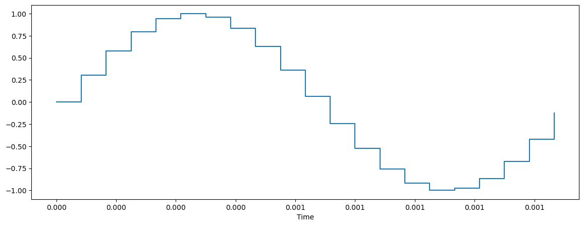
# plt로 표시
plt.figure(figsize=(14, 5))
plt.plot(range(a_cycle_time), sound_contents[:a_cycle_time], 'o-')
plt.show()

Out [26]:

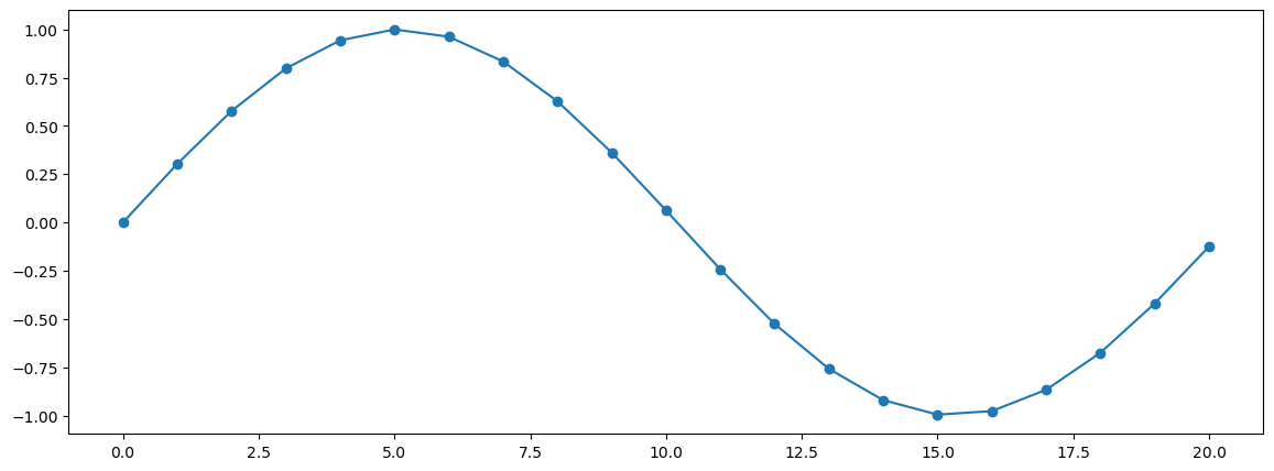
librosa 그래프는 realtime으로 표시!

주파수 구해보기

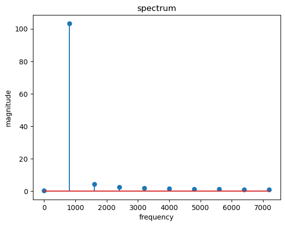
In [27]:

X = np.fft.fft(sound_contents[:a_cycle_time]*10) # 일반적으로 음성 분석에선 10ms 단위로 주파수 분석을 하면 적당함
mag = np.abs(X)
f = np.linspace(0, file_sampling_rate, len(mag))
f_left = f[:len(mag)//2]
spectrum_X = mag[:len(mag)//2]

plt.stem(f_left, spectrum_X, 'o-')
plt.xlabel('frequency')
plt.ylabel('magnitude')
plt.title('spectrum')
plt.show()

Out [27]:

In [28]:

spectrum_X

Out [28]:

array([  0.37506104, 103.33842577,   4.19259441,   2.37350619,
         1.72770691,   1.39521643,   1.19828769,   1.07409182,
         0.9941707 ,   0.94708465])

첫 magnitude 이후 배음의 존재 확인가능

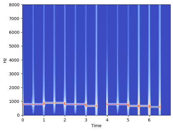
freq power spectrogram

librosa로 주파수 보기

In [29]:

X = librosa.stft(sound_contents) # short time fourir transform (10ms)
Xdb = librosa.amplitude_to_db(abs(X))
librosa.display.specshow(Xdb, sr=file_sampling_rate, x_axis='time', y_axis='hz')
plt.show()

Out [29]:

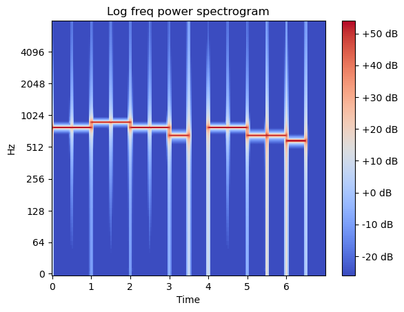
log scale
로그 적용으로 값이 있는 부분만 보기

In [30]:

X = librosa.stft(sound_contents) # short time fourir transform (10ms)
Xdb = librosa.amplitude_to_db(abs(X))
librosa.display.specshow(Xdb, sr=file_sampling_rate, x_axis='time', y_axis='log')
plt.title('Log freq power spectrogram')
plt.colorbar(format='%+2.0f dB')
plt.show()

Out [30]:

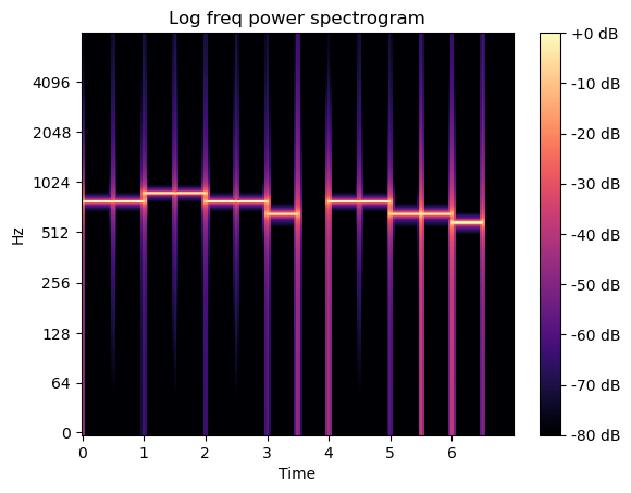
reference로 max값을 줘서 0dB부터 내려갈 수 있도록 재조정
0dB가 넘어가면 깨짐

In [31]:

X = librosa.stft(sound_contents) # short time fourir transform (10ms)
Xdb = librosa.amplitude_to_db(abs(X), ref=np.max)
librosa.display.specshow(Xdb, sr=file_sampling_rate, x_axis='time', y_axis='log')
plt.title('Log freq power spectrogram')
plt.colorbar(format='%+2.0f dB')
plt.show()

Out [31]:

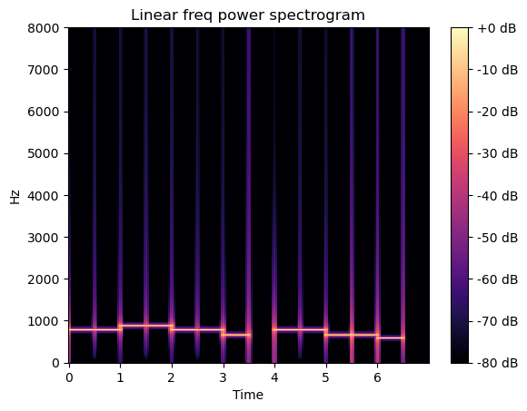
linear로 보기

In [32]:

X = librosa.stft(sound_contents) # short time fourir transform (10ms)
Xdb = librosa.amplitude_to_db(abs(X), ref=np.max)
librosa.display.specshow(Xdb, sr=file_sampling_rate, x_axis='time', y_axis='linear')
plt.title('Linear freq power spectrogram')
plt.colorbar(format='%+2.0f dB')
plt.show()

Out [32]:

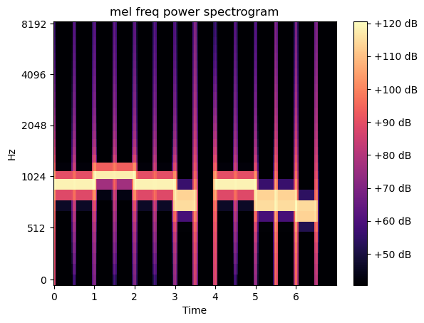
melspectrogram

In [33]:

D = abs(librosa.stft(sound_contents))
mel_spec = librosa.feature.melspectrogram(S=D, n_mels=30) # n_mels: 적절한 구분으로 구간을 나눔
mel_db = librosa.amplitude_to_db(mel_spec, ref=0.000001)

librosa.display.specshow(mel_db, sr=file_sampling_rate, x_axis='time', y_axis='mel')
plt.title('mel freq power spectrogram')
plt.colorbar(format='%+2.0f dB')
plt.show()

Out [33]:

Twitter Facebook LinkedIn

Kwak Jisub

음성 처리 - 사운드 툴

Sound Tools

IPython.ipd

악기 합성

노래 합성

soundfile

librosa

freq power spectrogram

melspectrogram

공유하기

댓글남기기

참고

python max 함수의 매개변수

python round 함수의 문제

python set 자료형과 메소드

MySQL GROUP BY와 MAX